SMOS delivers the first ever global map of Sea Surface salinity from Space close to GODAE requirements
Six months after switch on of the SMOS instrument Nicolas Reul from Ifremer has produced in the framework of the Centre Aval de Traitement des Donnees SMOS (CATDS) the following sea surface salinity map. It is a level 3 product (1°X1° monthly value) obtained from SMOS data acquired during the month of May 2010. (for those interested you will find below all the necessary explanations.

 There are still some issues (RFI notably), but the comparison with ARGO data gives, for the Pacific Tropical areas an accuracy of the order of .0.26 psu which is already very close to the GODAE target. Understanding that since May the L1 processor and the SMOS calibration has been significantly improved, we can be very optimistic!
Explanations (Nicolas Reul -Ifremer Brest- CATDS)
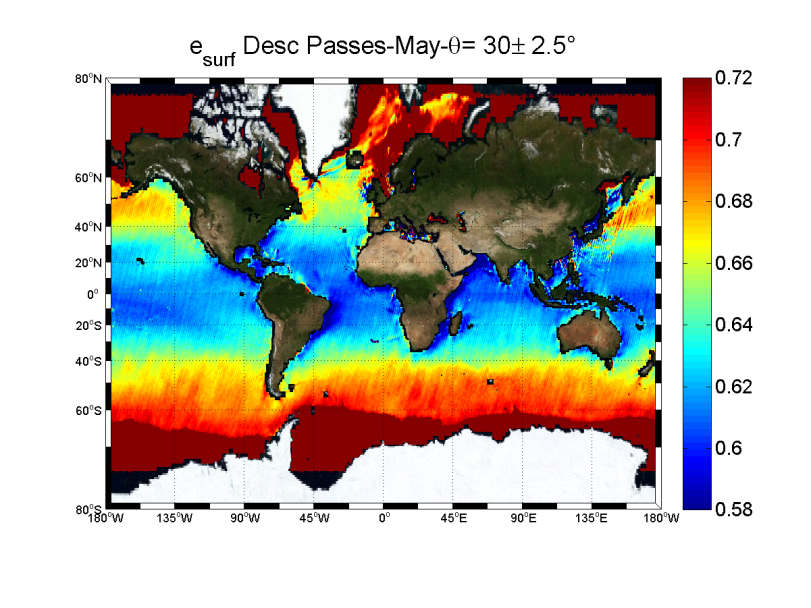
SMOS L1B brightness temperature data (generated by the DPGS Operational Processor v313) were collected at several 5°-wide multi-incidence angle bands within the alias-free field of view domain of the MIRAS antenna frame, for the complete month of May and over the world oceans. A ‘pseudo’ First Stokes parameter was evaluated from these data collection by summing successively acquired co-polar antenna brightness temperature measurements Tx and Ty (separated in dual polarization by 1.2 s). Analysis of the total power parameter instead of the individual X and Y -polarized data was chosen to minimize potential effects of the Faraday rotation across the ionosphere and to avoid antenna to surface frame transformation. The resulting First Stokes parameters (measured at the antenna altitude) were then corrected for modeled atmospheric effects and contributions from extra-terrestrial radiation reflected by the sea surface toward the MIRAS sensor. Given the coincident Sea Surface Temperature estimates from ECMWF products, the total power emissivity at the surface level along the orbit tracks was further evaluated. Data were finally best filtered for radio-frequency interferences using a mitigation technique based on the geophysical value of surface emissivity horizontal gradients, global histogram bounds and temporal variability thresholds. Composite maps of the estimated surface total power emissivity were then derived for each incidence angle bands, accumulating data over the month of May and averaging the data at several spatial resolutions varying from 0.25° to 1°. An example 0.5°x0.5° monthly-composite surface emissivity map from SMOS for May 2010 is given in the left figure below. It’s is a composite of data acquired during descending passes and for incidence angles between 27.5° and 32.5°.
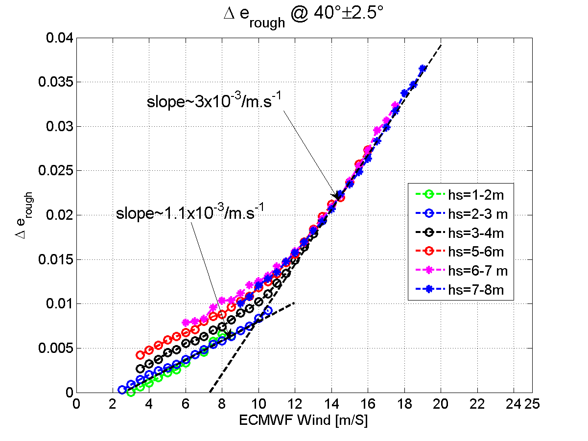
As illustrated in the plot of the above figure, showing bin-averaged data for incidences around 40° whatever SSS and SST values, a preliminary empirical multi-angular roughness correction algorithm could be derived based on the behavior of the surface emissivity as function of ECMWF wind speeds and WAM model wave heights. The roughness effect is seen to exhibits two linear major and distinct regimes: 1) low and moderate winds below 10-12 m/s and 2) wind speed stronger than ~ 12 m/s above which foam induced by breaking waves may additionally contribute to emissivity. Note that a clear dependence with sea surface heights is found in the low to moderate wind speed regime. Finally, sea surface salinity was retrieved from the multi-angular roughness-corrected data minimizing the difference between ‘flat’ ocean surface emissivity estimates from SMOS data and flat model predictions. The along-track retrieved SSS were then just averaged at the different spatial resolutions over the month.
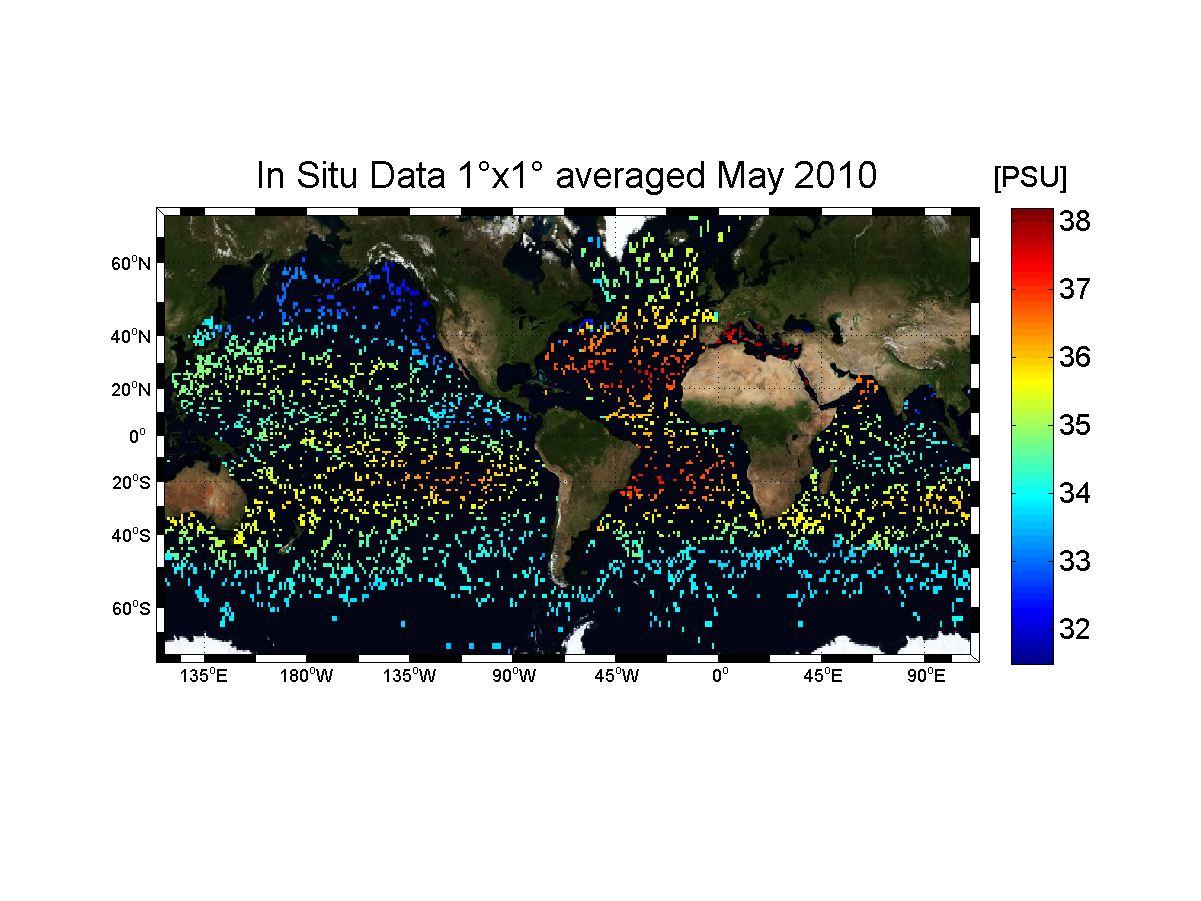
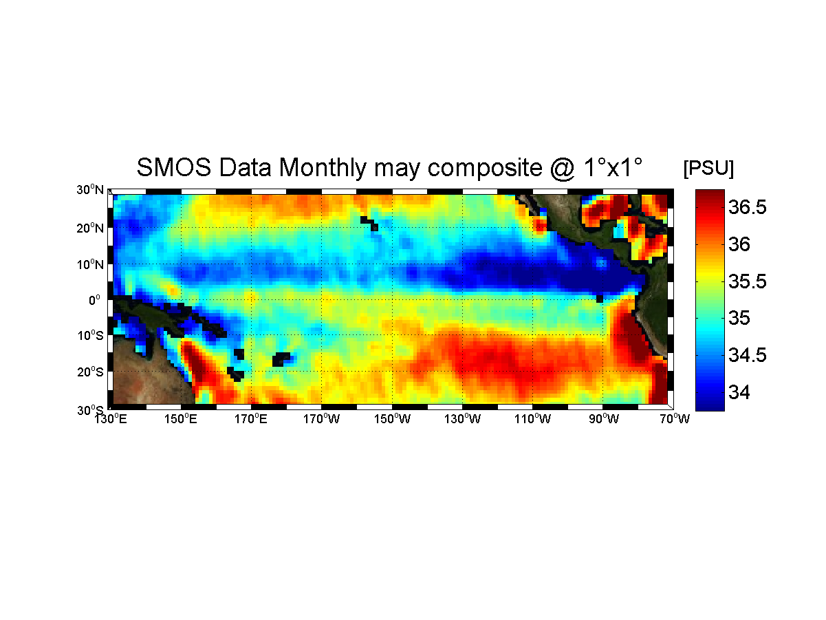
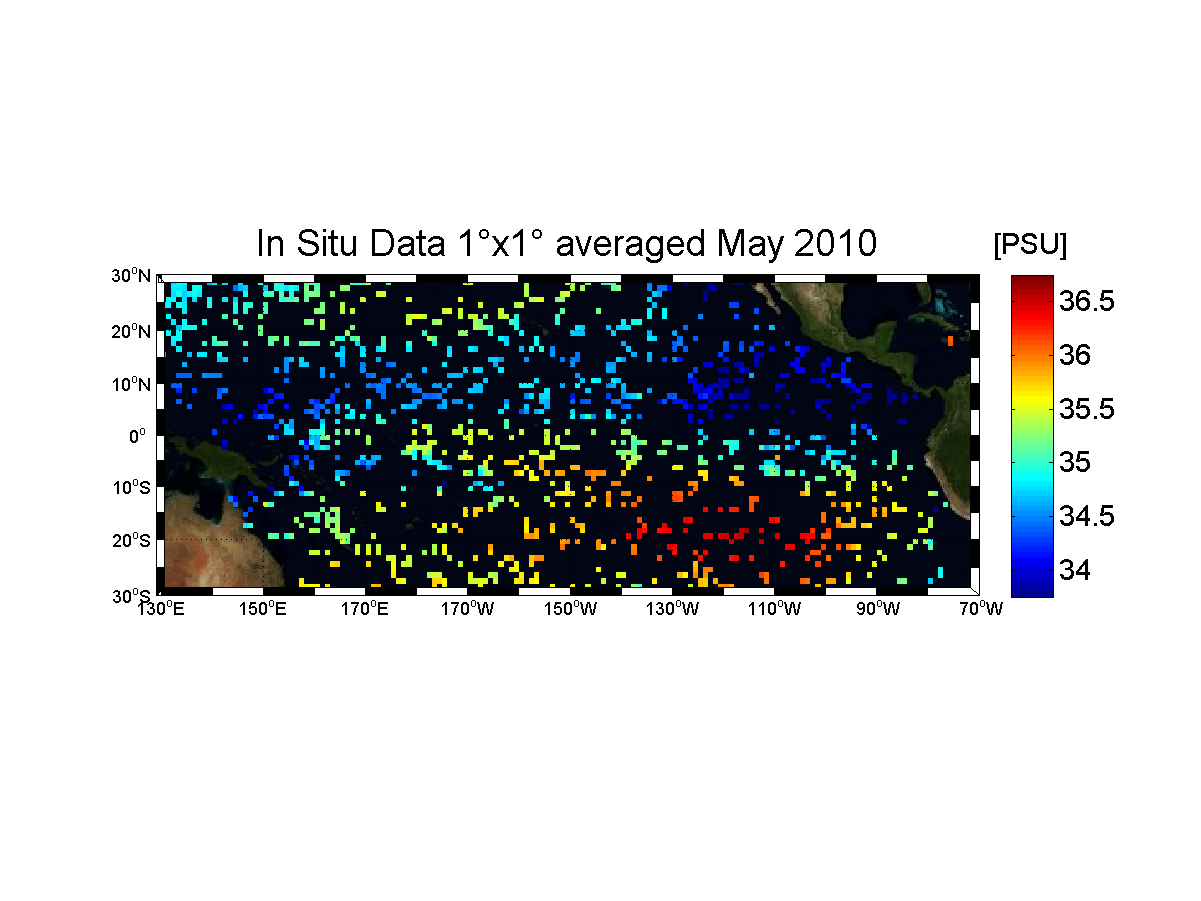
An example of monthly composite SSS charts solely based on SMOS ascending passes data is given below with a spatial resolution of 1°x1°. Upper ocean levels in situ SSS measurements (mostly acquired by Argo profilers, CTD sections and moorings) were collected and qualified by the GLOSCAL project for that same month and spatially averaged at a 1°x1° spatial resolution. The corresponding in situ data map is shown here below the SMOS chart for illustration.
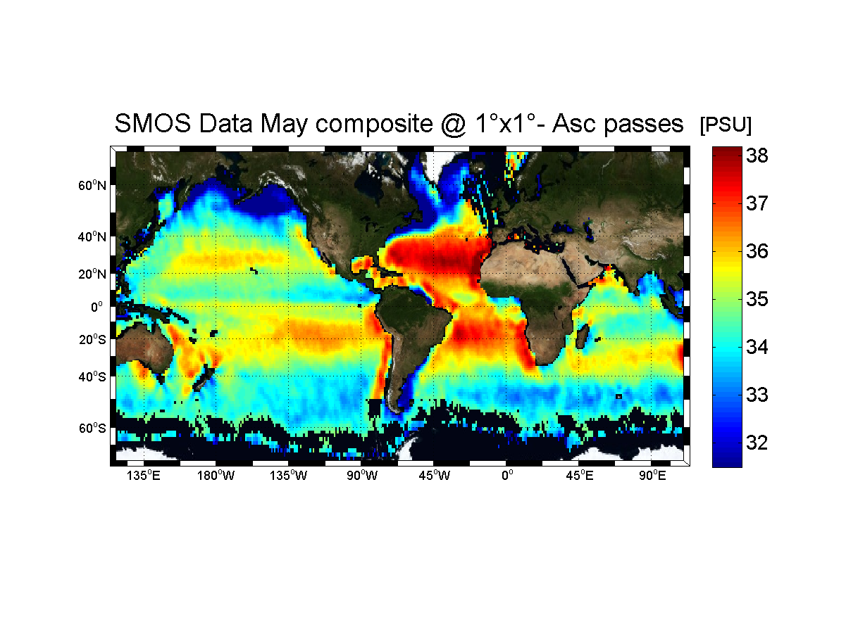
Note that erroneous (too salty) retrieved salinities were found at the averaged sea ice locations around Antarctica and were filtered out in this map. As well, clearly detectable pattern errors are found to form too salty bands along the west coast of the continents. A detailed analysis revealed that such non-geophysical signals is permanently found in the reconstructed brightness temperature data generated by the level1 operational processor version 313. While the exact reason is not yet found, this spurious signal is apparently no more detected in the new SMOS L1 data produced since the 7th of July, date at which the new version (v314) of the level1 processor was activated.
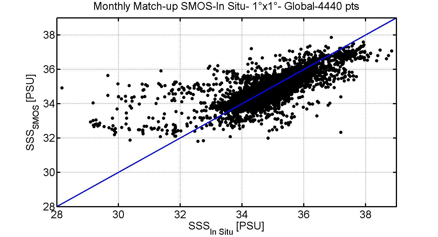 Given this probable artifact in level 1 processor, comparison with in situ data (figure above) nevertheless reveals an overall rms difference of about 0.4 psu between SMOS ascending orbit monthly averaged SSS @ 1°x1° resolution and in situ observations. Zoomed charts of the tropical Pacific SMOS SSS and in situ data is given below:
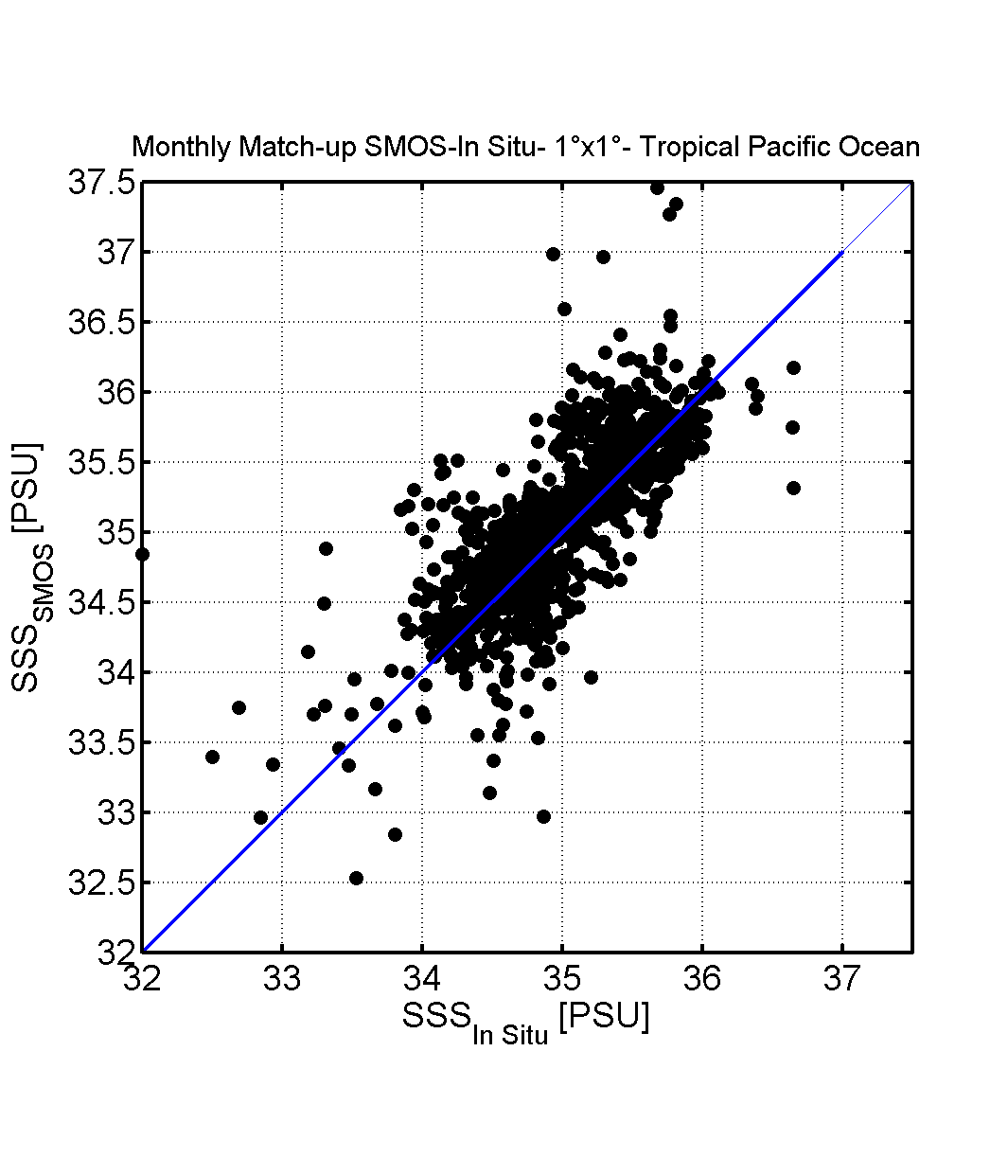
Accuracy of that SMOS data composite in the Pacific Tropical band is found to be 0.26 psu.
These results are very encouraging given the used SMOS data processor version level and the fact that only half the acquired data (ascending passes) were used here for the illustration.